Explaining the Pop-Out Variances as
Observed in the Study by Treisman and Gormican 1988
The following is a summary
of how the decomposition output can explain the variances observed in the visual
search studied by Treisman and Gormican (1988). It is emphasized, that we
solely interpret the ‘variances’; it is not meant to support the
feature-integration theory derived by Treisman. In contrary, our goal is to
argue that these pop-out phenomena evidence a parametric structural analysis,
which is based on dynamic processes and not on feature template detection.
The geometric contour
parameters are called orientation, length, degree of curvature (b), degree of inflexion (t), edginess (e), wiggliness (w) and
degree of isolation (r):
c(o, l, b, t, e, w, r).
The geometric sym-axis
(area) parameters are initial and end distance (s1 and s2),
angle (α), average distance (sm), elongation (e), flexion distance and flexion
location (sfx, pfx),
curvature and orientation:
a(s1, s2, α, sm,
e, sfx, pfx, b, o).
Note: For
a typical search display the SAT will not only generate sym-axes describing the
local configuration of structure, but also sym-axes describing the area between
elements. But because in a typical search task the subject is asked to focus on
the local elements only, those ‘between-feature’ sym-axis segments are
neglected. Thus, the following explanations consider local structure only.
The following figure numbers
refer to the figure numbers in their seminal paper (1988).
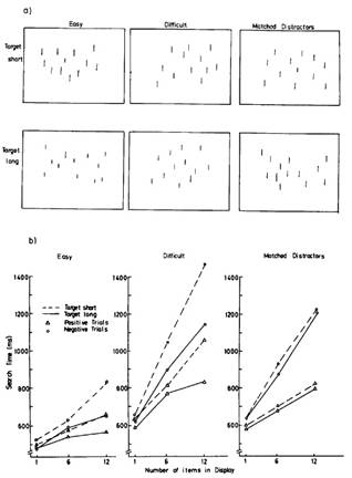
Figure 2: a deviation in the
length dimension l of the contour
descriptors.
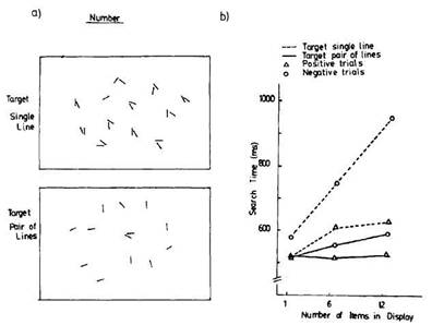
Figure 3: presence/absence
of a symmetric axis.
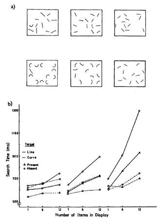
Figure 5: a deviation in the
bendness dimension b of the contour
vector.
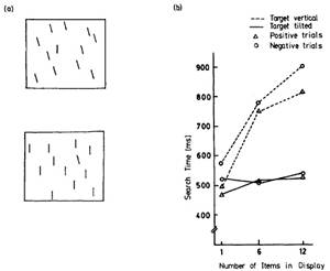
Figure 6: a deviation in the
orientation dimension o of the
contour vector.
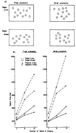
Figure 7: a deviation in the
elongation dimension of the sym-axis vector (e=0 for circles); there is also a deviation in contour lengths,
because a circle consists of a long, single contour, whereas an ellipse
consists of two shorter contours (after segregation).
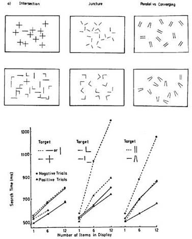
Figure 10:
- Intersection: can be
explained by the absence and presence of a group of sym-axis segments whose
starting points (s1) are
proximal, but such grouping has not been modeled in this study.
- Juncture: this can be
interpreted as the presence or absence of a deflection, that is a deviation of
the dimensions sfx and pfx of the sym-axis vector
from their default values (center point).
- Parallel vs. Converging: a
deviation of the sym-axis dimensions s1
and s2 or simply of the
angle α.
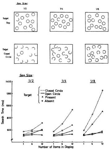
Figure 11:
- ½: presence and absence of
a sym-axis.
- ¼ and 1/8: presence or
absence of a sym-axis; or a deviation in contour length.
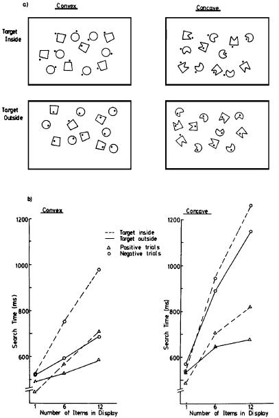
Figure 12: A deviation in
the context of a sym-axis (presence/absence of neighboring sym-axes):
A point outside and near a
shape generates a sym-axis which is relatively isolated as opposed to a sym-axis
generated by a point inside, that is connected to sym-axes describing the
entire shape. Contextual information has not been modeled yet explicitly in our
models.
Discriminating parallel/serial
The distinction between
parallel and serial appears to have three reasons:
1) A varying degree in the
deviation, e.g. figure 5.
2) Two dimensions are
different in the same visual display, e.g. finding a circle amongst ellipses of
different orientations (upper right, figure 7).
3) A deviation of one
dimension to one side of the scale, for instance it seems easier to find a
larger distance e2 than a
smaller one, e.g. figure 10, parallel vs. converging.
The distinction between
serial and parallel is not particularly considered in the following
implementation and categorization analysis, as we do not aim at an emulation of
saliency but rather at an exploration of the issue of representation.